複数回答(multiple answer, MA)の集計表をコレスポンデンス分析にかけて大丈夫？

結論から言うと、大きな問題はなさそうです。

複数回答とは？

ブランドのイメージなどを聞くアンケートでは、「○○ブランドのイメージとして、あてはまるものをすべて選んでください」というような設問がよく使われます。

1つの設問に対して、複数の選択肢を選ぶことができる形式で、複数回答(multiple answer)、略してMAとも呼ばれます。

MAのコレポン問題

このタイプの質問の分析にはコレスポンデンス分析がよく使われます。

コレスポンデンス分析には集計表の周辺度数をかけ合わせた期待値が使われますが、複数回答の場合周辺度数が100%にはならない（回答者数が100%）ので、そのままコレポンにかけるのはマズいのでは？？？というのが実は長年の疑問でした。

そこで、こんなふうに考えてみました。

複数回答は、各選択肢毎単数回答（single answer）をまとめたものと解釈できる。

それであれば、各選択肢毎に選択、非選択の両方をカウントしたクロス集計表をもとにコレポンすれば問題ないんじゃないか？

検証してみる

検証のためのデータとして、GMOリサーチさんのデータを引用させていただきます。

「n=100」との記載がありますが、各セグメントごとにn=100と解釈しました。

library(tidyverse)
library(ggrepel)

##### データ整形
dat_MA <- matrix(
  c(
    13, 13,  8, 23, 16, 20,  3,  4,
    25, 13,  8, 23,  8, 10,  8,  5,
    28,  6,  7, 25,  7, 15,  5,  5,
     7,  8,  6, 38, 12, 21,  4,  4,
     8, 12, 24, 10,  9,  7, 28,  2,
    12, 20, 17, 18,  7,  6, 10, 10,
    15, 21, 19, 15,  4, 12,  4, 10,
     5,  9, 10, 29, 17, 19,  8,  3
    ),
  ncol = 8,
  byrow = TRUE,
  dimnames = list(
    性年代 = c(
      "20代男性", "30代男性", "40代男性", "50代男性",
      "20代女性", "30代女性", "40代女性", "50代女性"
      ),
    コンビニで買うお昼ご飯 = c(
      "おにぎり類", "パン類", "サンドイッチ", "弁当類",
      "パスタ類", "ラーメン・うどん類", "野菜・サラダ類", "冷凍食品類"
      )
    )
  )
  
dat_SA <- cbind(
  dat_MA,
  100 - dat_MA
  ) 

dimnames(dat_SA)[[2]] <- c(
  paste0("y_", dimnames(dat_MA)[[2]]),
  paste0("n_", dimnames(dat_MA)[[2]])
  )

dat_SA

これで各選択肢の選択(y)、非選択(n)をまとめたクロス集計表ができました。

コレポンする

従来の選択項目のみをカウントした集計表と、選択、非選択をまとめたクロス集計表を、それぞれコレスポンデンス分析にかけ、比較してみます。

library(ca)

res.ca_MA <- ca(dat_MA) # 選択項目のみの従来型
res.ca_SA <- ca(dat_SA) # 選択、非選択をまとめたSA型

summary(res.ca_MA)
summary(res.ca_SA)

res.plot.ca_MA <- plot(res.ca_MA, main = "MA", map = "symbiplot", arrows = c(TRUE, TRUE))
res.plot.ca_SA <- plot(res.ca_SA, main = "SA", map = "symbiplot", arrows = c(TRUE, TRUE))

行要素の比較

MAとSAの行要素について、コレポンの結果を比較してみます。

f:id:bob3:20220227161143p:plain

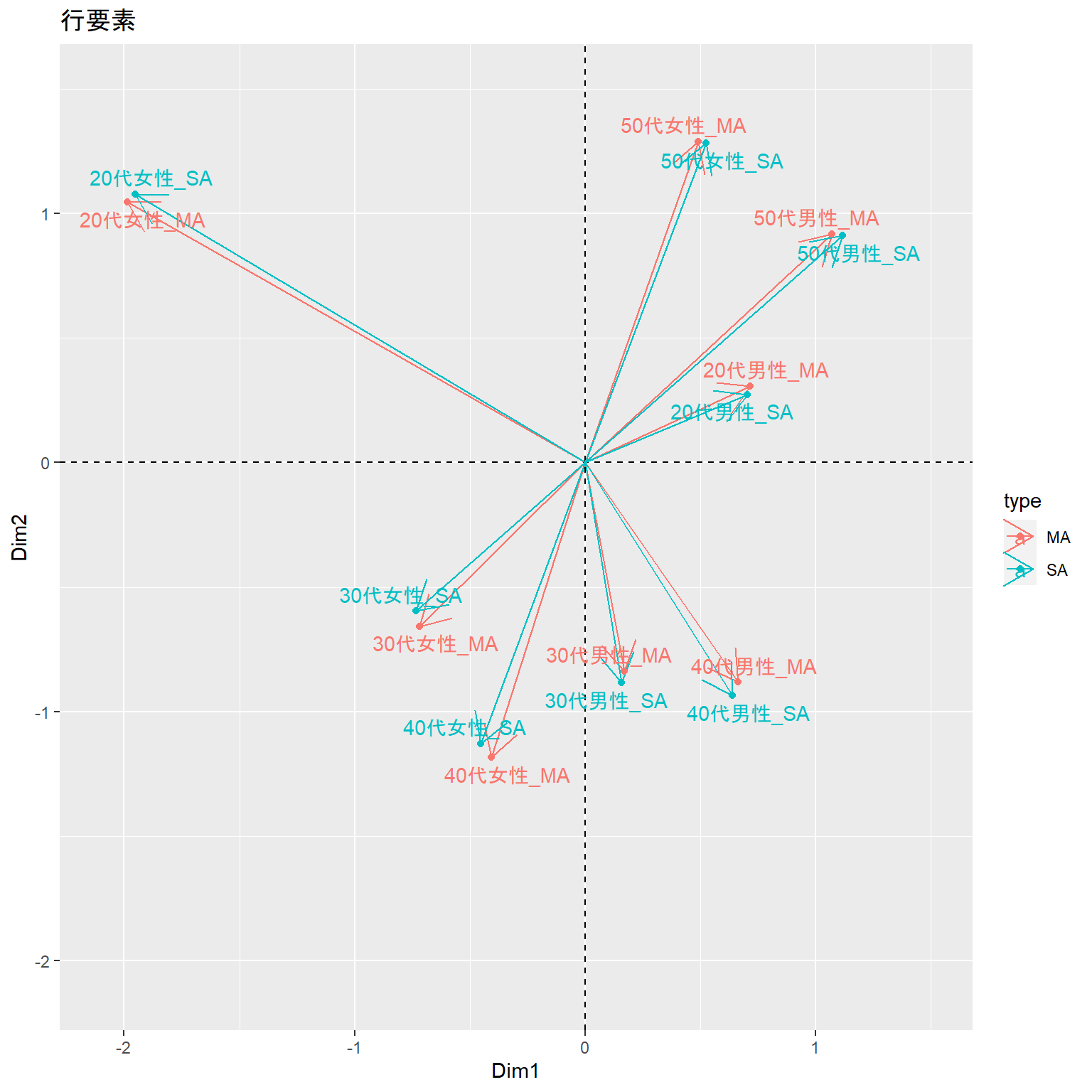
微妙にずれますが、ほぼ同じと解釈してもよさそうです。

res.plot.ca_MA$rows %>%
  as.data.frame() %>%
  rownames_to_column() %>%
  mutate(
    rowname = paste0(rowname, "_MA"),
    Dim1 = scale(Dim1),
    Dim2 = scale(Dim2),
    type = "MA"
    ) %>%
  bind_rows(
    res.plot.ca_SA$rows %>%
      as.data.frame() %>%
      rownames_to_column() %>%
      mutate(
        rowname = paste0(rowname, "_SA"),
        Dim1 = scale(Dim1),
        Dim2 = scale(0 - Dim2), #x軸を反転
        type = "SA"
        )
    ) %>%
  ggplot(aes(x=Dim1, y=Dim2, label = rowname, color=type)) +
  scale_x_continuous(limits = c(-2.1, 1.5)) +
  scale_y_continuous(limits = c(-2.1, 1.5)) +
  geom_hline(yintercept = 0, linetype = 2) +
  geom_vline(xintercept = 0, linetype = 2) +
  geom_segment(aes(x=0, y=0, xend=Dim1, yend=Dim2), arrow = arrow(type = "open")) +
  geom_point() +
  geom_text_repel() +
  labs(title = "行要素")

列要素の比較

こんどは列要素について、比較してみます。

f:id:bob3:20220227161213p:plain

こちらも微妙にずれますが、ほぼ同じと解釈してもよさそうです。

# 列要素 ほぼ一致
res.plot.ca_MA$cols %>%
  as.data.frame() %>%
  rownames_to_column() %>%
  mutate(
    rowname = paste0(rowname, "_MA"),
    Dim1 = scale(Dim1),
    Dim2 = scale(Dim2),
    type = "MA"
  ) %>%
  bind_rows(
    res.plot.ca_SA$cols %>%
      as.data.frame() %>%
      rownames_to_column() %>%
      slice(1:8) %>%
      mutate(
        rowname = paste0(rowname, "_SA"),
        Dim1 = scale(Dim1),
        Dim2 = scale(0 - Dim2), #x軸を反転
        type = "SA"
    )
  ) %>%
  ggplot(aes(x=Dim1, y=Dim2, label = rowname, color=type)) +
  scale_x_continuous(limits = c(-2, 1.25)) +
  scale_y_continuous(limits = c(-2, 1.25)) +
  geom_hline(yintercept = 0, linetype = 2) +
  geom_vline(xintercept = 0, linetype = 2) +
  geom_segment(aes(x=0, y=0, xend=Dim1, yend=Dim2), arrow = arrow(type = "open")) +
  geom_point() +
  geom_text_repel() +
  labs(title = "列要素")

結論

ということで、MAの集計表をそのままコレポンにかけても実用上は問題なさそうです。