Rで構造方程式モデリング(共分散構造分析)を実行する場合、semパッケージかlavaanパッケージを使うことが多いです。
https://socialsciences.mcmaster.ca/jfox/Misc/sem/index.htmlsocialsciences.mcmaster.ca
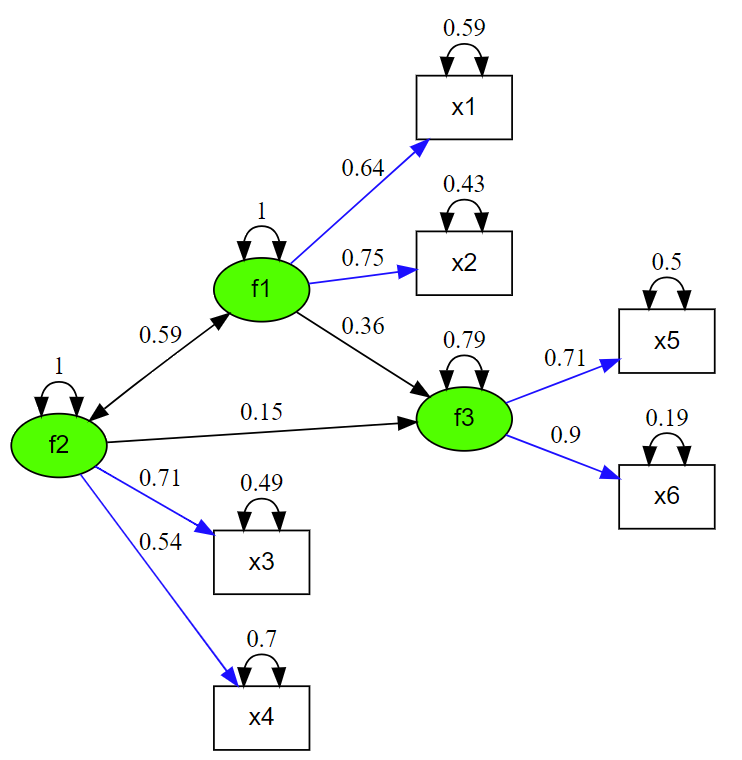
構造方程式モデリングを実施したらパス図が書きたくなります。
semパッケージやlavaanパッケージで作ったモデルからパス図を描くパッケージとしてsemPlotパッケージがありますが、なんかしっくりこない。
http://sachaepskamp.com/documentation/semPlot/semPaths.htmlsachaepskamp.com
そこで自分で lavaan のモデルからDiagrammeRを利用してキレイなパス図を描く関数を作りました。
rich-iannone.github.io
my_lavaan_plot <- function(fit, standardized = TRUE) {
  require(lavaan)
  require(stringr)
  require(dplyr)
  require(DiagrammeR)

  #描画に必要なパラメータをdfとして取り出す
  pars <- parameterEstimates(fit,
                             standardized = standardized)
  # エッジ(パス)の設定、"=~"を抜き出しpaseteして因子負荷量
  temp01 <- dplyr::filter(pars, op == "=~")
  temp02 <- str_c('  \"', temp01$lhs,'\"', ' -> ','\"', temp01$rhs, '\"',
                  '[label=\"', round(temp01$std.all,2),
                  '\" color=blue penwidth=1.001];')
  # "~"を抜き出しpaseteして因子間回帰
  temp31 <- dplyr::filter(pars, op == "~")
  temp32 <- str_c('  \"', temp31$rhs,'\"', ' -> ','\"', temp31$lhs, '\"',
                  '[label=\"', round(temp31$std.all,2),
                  '\" color=black penwidth=1.001];')
  # "~~"抜き出す
  temp11 <- dplyr::filter(pars, op == "~~")
  temp12 <- str_c('  \"', temp11$rhs,'\"', ' -> ','\"', temp11$lhs, '\"',
                  '[label=\"', round(temp11$std.all,2),
                  '\" color=gray penwidth=1.001, dir = both];')
  # ノードの設定 観測変数と潜在因子
  temp00 <- inspect(fit)$lambda
  test.f <- colnames(temp00) #潜在因子
  test.v <- rownames(temp00) #観測変数
  temp21 <- str_c('  \"', test.f,'\" [fontname=\"Helvetica\" fontsize=14 fillcolor = green shape=ellipse style=filled];')
  temp22 <- str_c('  \"', test.v,'\" [fontname=\"Helvetica\" fontsize=14 fillcolor=\"transparent\" shape=box style=filled];')
  tempALL <- c('digraph \"res.s\" {',
               '  layout = dot;', #dot, fdp
               '  rankdir=LR;',
               '  size=\"8,8\";',
               temp21,
               temp22,
               temp02,
               temp32,
               '  center=1;',
               temp12,
               '}')

  grViz(tempALL)
}
使い方はlavaanで作ったモデルを食わせるだけ。
# テスト用のモデル
# ヘッドスタート計画の相関係数行列
HS <- matrix(c(1.000, 0.484, 0.224, 0.268, 0.230, 0.265,
               0.484, 1.000, 0.342, 0.215, 0.215, 0.295,
               0.224, 0.342, 1.000, 0.387, 0.196, 0.234,
               0.268, 0.215, 0.387, 1.000, 0.115, 0.162,
               0.230, 0.215, 0.196, 0.115, 1.000, 0.635,
               0.265, 0.295, 0.234, 0.162, 0.635, 1.000), 6)
colnames(HS) <- rownames(HS) <- paste("x", 1:6, sep="")

HS.mdl.2 <- '
  # 測定方程式
  f1 =~ x1 + x2
  f2 =~ x3 + x4
  f3 =~ x5 + x6
  # 構造方程式
  f3 ~  f1 + f2 '
fit <- sem(HS.mdl.2, sample.cov=HS, sample.nobs=1800)
summary(fit, fit.measures=TRUE, standardized=TRUE)

my_lavaan_plot(fit)