『データ可視化学入門』をRで書く 2.3 標本を視えるようにする

2.3 標本を視えるようにする

この記事はR言語 Advent Calendar 2023 シリーズ2の7日目の記事です。
[qiita.com

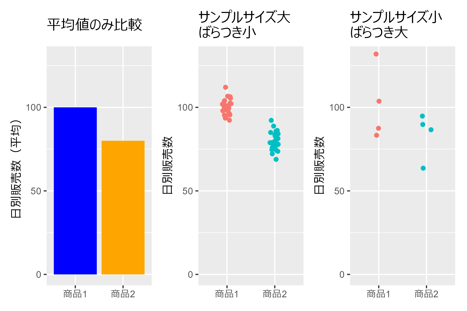
2.3.1 平均値の棒グラフの危険性

##### 2.3.1 #####
library(tidyverse)

p1 <- data.frame(
  x = c("商品1","商品2"),
  avg = c(100, 80)
  ) |>
  ggplot(aes(x = x, y = avg)) +
  geom_col(fill = c("blue","orange")) +
  theme(axis.title.x = element_blank()) +
  labs(y = "日別販売数（平均）", title = "平均値のみ比較") +
  coord_cartesian(ylim = c(0, 130))

# データの生成
n_small <- 30
n_large <- 4
set.seed(0)
df_small_var <- bind_rows(
  data.frame(
    商品 = rep("商品1", n_small),
    日別販売数 = rnorm(n_small, 100, 5) # 平均100、標準偏差5の正規分布に従う乱数を30個生成
    ), 
  data.frame(
    商品 = rep("商品2", n_small),
    日別販売数 = rnorm(n_small, 80, 5) # 平均80、標準偏差5の正規分布に従う乱数を30個生成
    )
  ) 

p2 <- df_small_var |>
  ggplot(aes(x=商品, y=日別販売数, color = 商品)) + 
  geom_jitter(width = 0.1, height = 0) +
  theme(
    axis.title.x = element_blank(),
    legend.position = "none"
    )+
  labs(title = "サンプルサイズ大\nばらつき小") +
  coord_cartesian(ylim = c(0, 130))

set.seed(1)
df_large_var <- bind_rows(
  data.frame(
    商品 = rep("商品1", n_large),
    日別販売数 = rnorm(n_large, 100, 20) # 平均100、標準偏差20の正規分布に従う乱数を4個生成
  ),
  data.frame(
    商品 = rep("商品2", n_large),
    日別販売数 = rnorm(n_large, 80, 20) # 平均80、標準偏差20の正規分布に従う乱数を4個生成
  )
)

p3 <- df_large_var |>
  ggplot(aes(x=商品, y=日別販売数, color = 商品)) + 
  geom_jitter(width = 0.1, height = 0) +
  theme(
    axis.title.x = element_blank(),
    legend.position = "none"
  )+
  labs(title = "サンプルサイズ小\nばらつき大") +
  coord_cartesian(ylim = c(0, 130))

p1 + p2 + p3

2.3.1

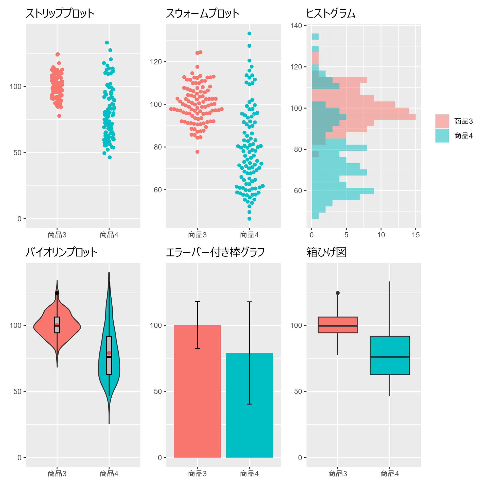
2.3.2 様々な標本の可視化

##### 2.3.2 #####
library(tidyverse)
library(ggbeeswarm)
library(Hmisc)
library(patchwork)

set.seed(0) # 乱数のシードを設定（再現性のため）
num_samples <- 100 # サンプルサイズ

# データフレームの生成
data <- data.frame(
  Value = c(
    rnorm(num_samples, 100, 10), # 平均100、標準偏差10の正規分布
    rnorm(num_samples, 80, 20)   # 平均80、標準偏差20の正規分布
    ),
  Category = c(
    rep("商品3", num_samples), 
    rep("商品4", num_samples)
    )
  )

# ggplot2の基本設定
plt <- data |>
  ggplot(aes(x=Category, y=Value)) +
  theme(
    axis.title.x = element_blank(),
    axis.title.y = element_blank(),
    legend.position = "none"
  )

# ストリッププロット (Dodge position)
p1 <- plt +
  geom_jitter(aes(color = Category), height = 0, width = 0.1)+
  scale_y_continuous(limits = c(0, 140)) +
  labs(title = "ストリッププロット")

# スウォームプロット
p2 <- plt +
  geom_beeswarm(aes(color = Category),cex = 3) +
  labs(title = "スウォームプロット")

# ヒストグラム
p3 <- data |>
  ggplot(aes(y=Value, fill=Category)) +
  geom_histogram(alpha=0.5, position='identity') +
  labs(title = "ヒストグラム") +
  theme(
    axis.title.x = element_blank(),
    axis.title.y = element_blank(),
    legend.title = element_blank()
  )

# バイオリンプロット
p4 <- plt + 
  geom_violin(aes(fill = Category),trim=FALSE) +
  geom_boxplot(width = .1, fill = "gray", color="black")+
  stat_summary(fun = mean, geom = "point", 
               shape =16, size = 2, color = "red", alpha = 0.5)+
  scale_y_continuous(limits = c(0, 140))+
  labs(title = "バイオリンプロット")

# エラーバー付き棒グラフ
p5 <- plt +
  stat_summary(aes(fill = Category),fun = "mean", geom = "bar") +
  stat_summary(geom = "errorbar",
               fun.data = "mean_sdl",
               width = 0.1, color = "black") +
  scale_y_continuous(limits = c(0, 140))+
  labs(title = "エラーバー付き棒グラフ")

# 箱ひげ図
p6 <- plt +
  geom_boxplot(aes(fill = Category)) +
  scale_y_continuous(limits = c(0, 140))+
  labs(title = "箱ひげ図")

(p1 + p2 + p3) / (p4 + p5 + p6)

2.3.2

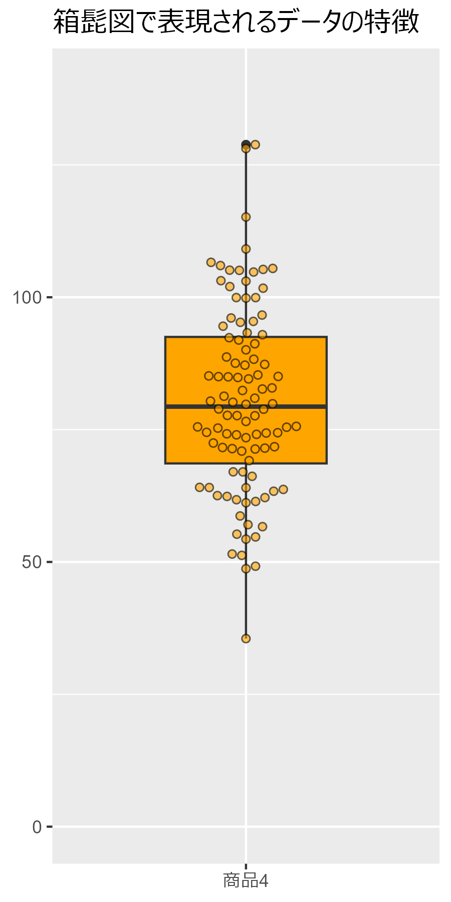
2.3.3 箱髭図の構成要素

##### 2.3.3 #####
library(tidyverse)
library(ggbeeswarm)

set.seed(0)# シード設定

data.frame(
  Value = rnorm(100, mean=80, sd=20),
  Category = "商品4"
  ) |>
  ggplot(aes(x=Category, y=Value)) +
  geom_boxplot(fill = "orange", width = 0.5) +
  geom_beeswarm(shape = 21, cex = 3, fill = "orange", alpha=0.6) +
  coord_cartesian(ylim = c(0,140)) +
  labs(title = "箱髭図で表現されるデータの特徴") +
  theme(
    legend.position="none", 
    axis.title.x=element_blank(), 
    axis.title.y=element_blank()
    )

2.3.3

第2章3節は以上です。